AI Series- Vector Databases Part 2: From Beginner to Pro

Part 2 of 4 in "Vector Databases: From Beginner to Pro."

Jul 13, 2026

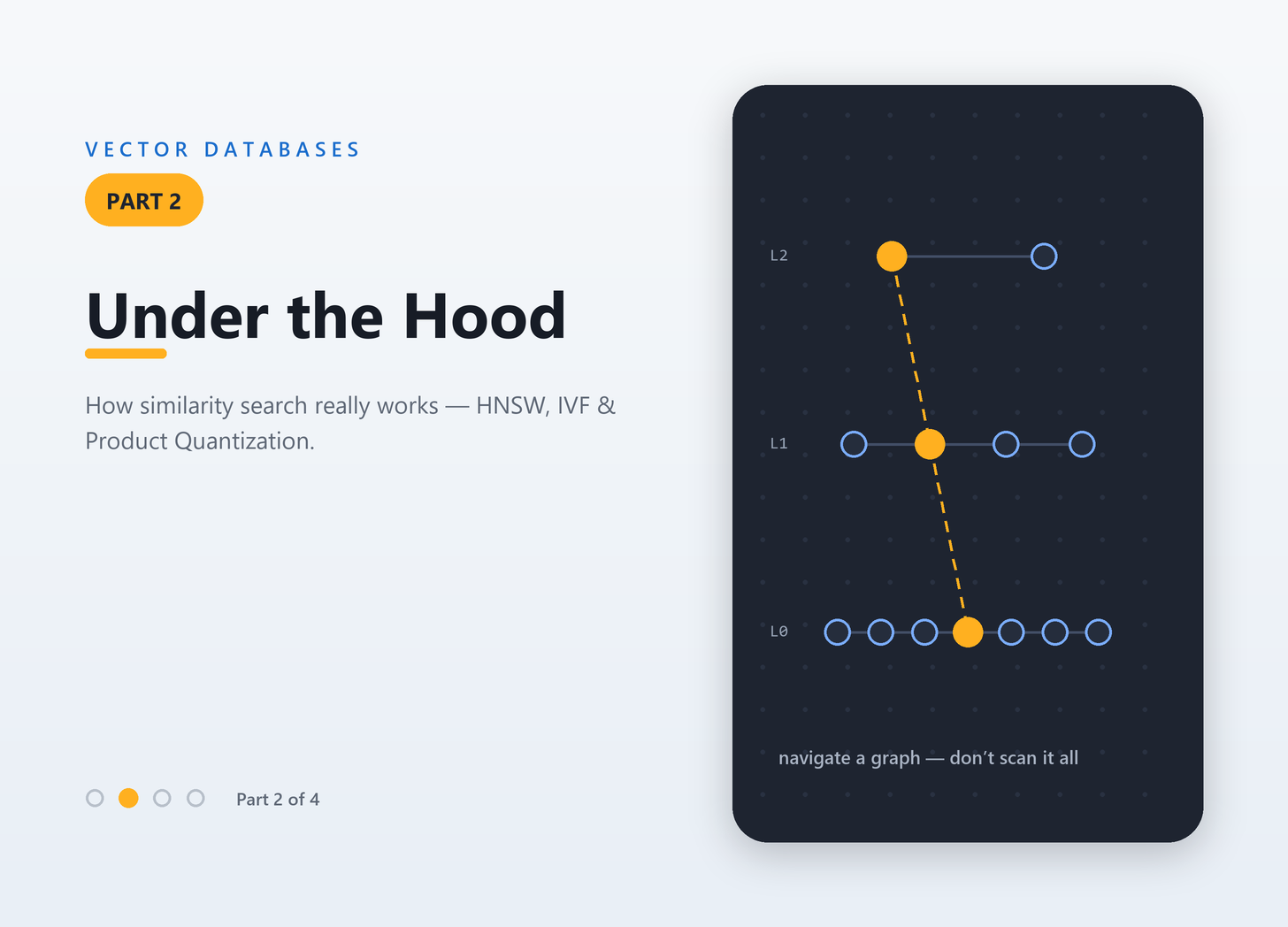
Part 2 — Under the Hood: How Vector Databases Actually Work

Part 2 of 4 in “Vector Databases: From Beginner to Pro.” If you haven’t read Part 1, start there — this post assumes you know what an embedding is and why “nearest neighbor search” is the core operation.

In Part 1 we ended on a cliffhanger: to find the vectors most similar to your query, the naive method is to compare against every vector in the database. That’s fine for a thousand vectors and hopeless for a hundred million.

So how does a vector database return the top 10 matches out of a billion in a few milliseconds — without looking at all of them?

That’s this whole post. We’ll build the answer in four layers:

How “similar” is measured (distance metrics)
Why exact search is doomed at scale (the curse of dimensionality)
The indexes that save us (HNSW, IVF, PQ) — with intuition, not just names
The rest of a real system (filtering, sharding, the tradeoff triangle)

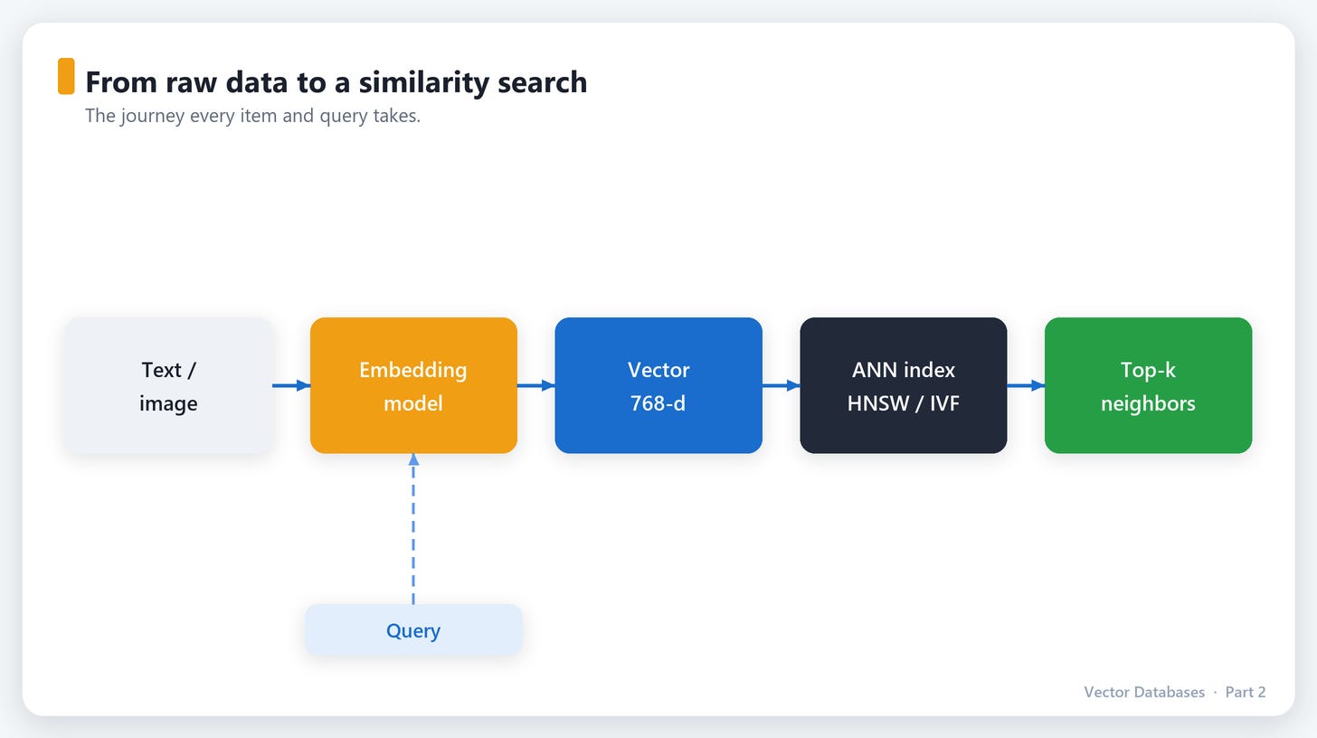
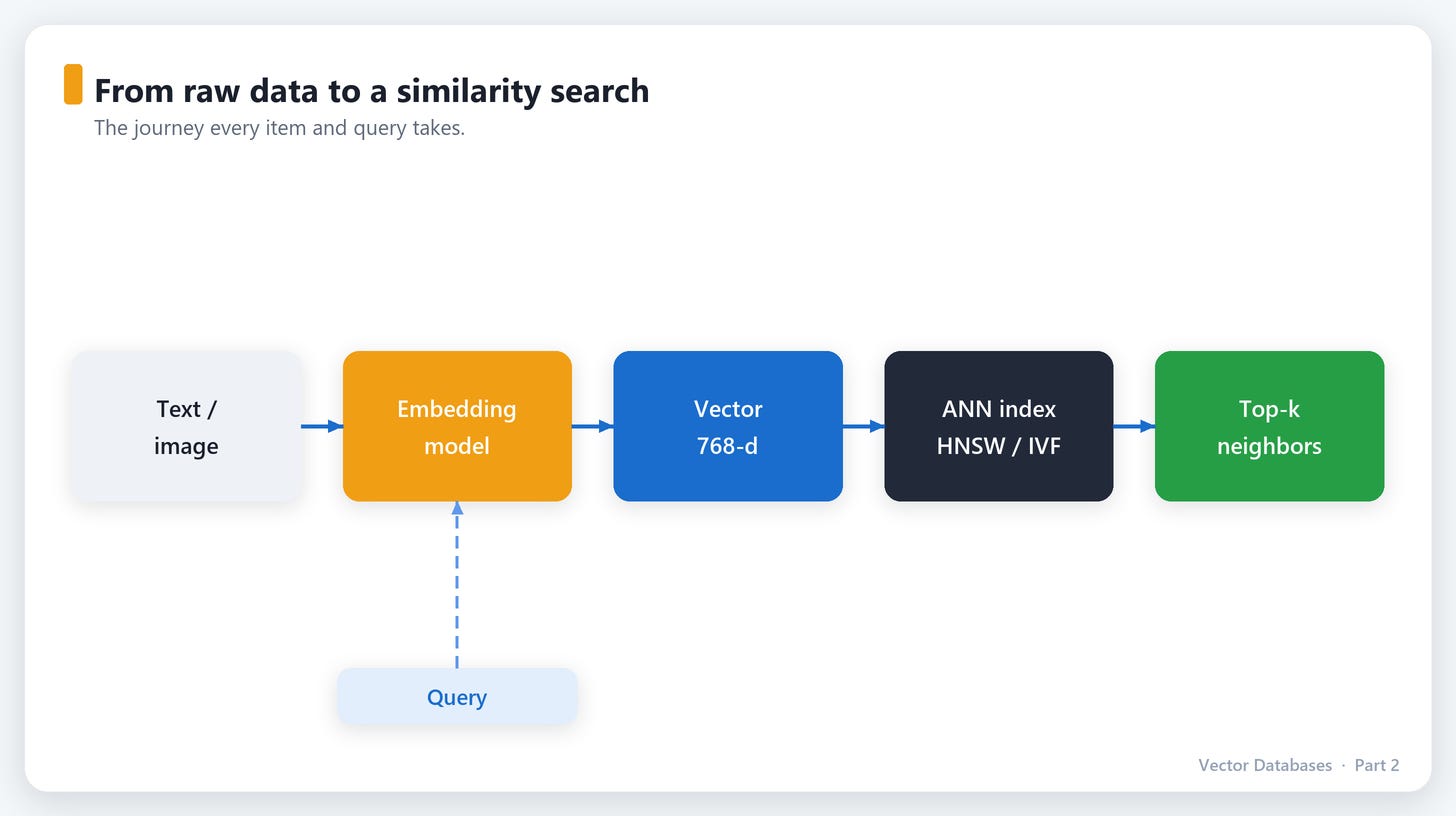
By the end you’ll understand the knobs that actually matter when your search is too slow, too inaccurate, or eating too much RAM.

Layer 1: How do we measure “similar”?

“Nearest neighbor” implies distance. But there are a few different ways to measure distance between two vectors, and picking the right one matters.

The three you’ll actually see

1. Euclidean distance (L2) — straight-line distance, the one from school. Small distance = similar.

d(a, b) = sqrt( Σ (aᵢ − bᵢ)² )

2. Cosine similarity — the angle between two vectors, ignoring their length. This is the most common choice for text embeddings, because we usually care about direction (meaning), not magnitude.

cosine(a, b) = (a · b) / (‖a‖ · ‖b‖)     range: −1 (opposite) … 1 (identical)

Intuition: two documents about the same topic point the same way even if one is longer. Cosine ignores length; Euclidean doesn’t.

3. Dot product (inner product) — like cosine but without normalizing for length, so magnitude matters. Fast, and common in recommender systems where “bigger = stronger signal” is intended.

a · b = Σ (aᵢ · bᵢ)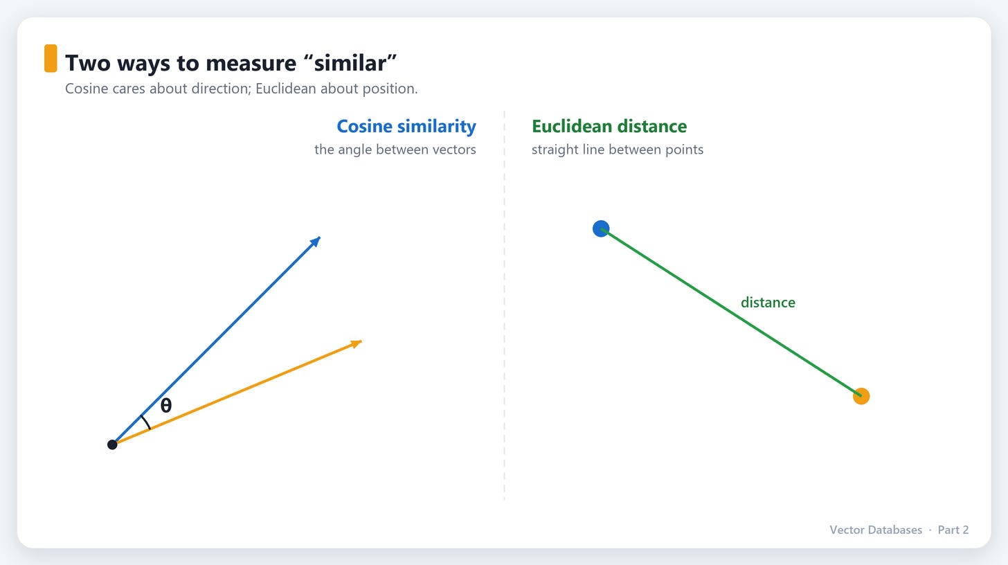

Which do I pick?

Use the metric your embedding model was trained/recommended for. This isn’t a preference — it’s a correctness requirement. Most modern text models (OpenAI, sentence-transformers) are tuned for cosine similarity. Use the wrong metric and your results quietly get worse.

Pro tip: If your vectors are normalized to unit length (‖v‖ = 1), then cosine similarity, dot product, and Euclidean distance all rank neighbors identically. Many systems normalize on ingest so they can use the fastest metric (dot product) while getting cosine’s behavior. When someone says “just normalize your vectors,” this is why.

Layer 2: Why exact search collapses at scale

Let’s be precise about the pain. Comparing a query to one vector of dimension d costs about d operations. Comparing to N stored vectors costs N × d.

N = 10,000,000 vectors
d = 768 dimensions
→ ~7.68 billion multiply-adds  PER QUERY

Now serve 1,000 queries per second. The arithmetic simply doesn’t close on a normal machine. And it gets worse than “linear and slow.”

The curse of dimensionality

In high-dimensional space, geometry stops behaving the way your 2D/3D intuition expects. Distances between points become weirdly uniform — everything starts to look roughly equidistant from everything else. Classic space-partitioning tricks that work great in 2D (like k-d trees) degrade until they’re no better than brute force once you’re in hundreds of dimensions.

So we can’t cheat with clever exact partitioning. We need a different bargain.

The bargain: give up “exact” for “almost always right”

Here’s the insight the whole industry runs on. In practically every real application — search, RAG, recommendations — you don’t actually need the mathematically guaranteed closest vectors. If the true top-10 and your returned top-10 overlap by 9 or 10 items, no user will ever notice.

So we relax the requirement:

Approximate Nearest Neighbor (ANN): find vectors that are almost certainly among the closest, by examining only a tiny fraction of the dataset.

The quality of an ANN index is measured by recall@k: of the true k nearest neighbors, what fraction did we actually return? Recall of 0.98 means we found 98% of the real top results — usually indistinguishable from perfect, at a fraction of the cost.

This trade — a sliver of accuracy for 100–1000× speed — is what makes billion-scale search feel instant. Now let’s look at how.

Layer 3: The indexes that make it fast

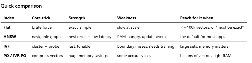
There are three big ideas. Real databases mix and match them. Understand these and you understand ~90% of every vector index in existence.

Index A: HNSW — the graph you navigate (the workhorse)

HNSW (Hierarchical Navigable Small World) is the default in most modern vector databases (Qdrant, Weaviate, Milvus, pgvector’s hnsw, Pinecone under the hood). If you learn one index, learn this one.

The intuition — a “six degrees of separation” map. Imagine every vector is a person, connected to a handful of others with similar meaning. To find who’s most similar to a query, you don’t poll everyone on Earth — you start at some person, hop to whichever of their friends is closest to the target, then to that person’s closest friend, and so on. You “walk” toward the answer, getting warmer each hop.

The “hierarchical” part — express lanes. A single flat friend-graph can get you stuck in the wrong neighborhood. So HNSW stacks layers:

Layer 2 (sparse):   A ─────────────── F           ← few nodes, long jumps
                     │                 │
Layer 1 (medium):   A ── C ─────── E ─ F ── H
                     │    │         │   │    │
Layer 0 (all nodes): A-B-C-D-E-F-G-H-I-J-K-L...    ← every vector, short hops

You enter at the top (few nodes, huge jumps) to teleport near the right region fast, then descend layer by layer, each one denser, refining your position — like zooming from country → city → street. It’s a skip-list for geometry.

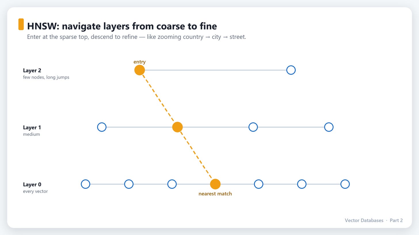
Why it wins: searches are roughly O(log N) instead of O(N). Excellent recall, very low latency.

The knobs (you’ll tune these for real):

M — neighbors per node. Higher = better recall + more memory.
ef_construction — how hard it works while building the graph. Higher = better index, slower builds.
ef_search (a.k.a. ef) — how many candidates to explore at query time. This is your live recall↔speed dial: raise it for better recall, lower it for lower latency.

The costs: the graph lives in RAM (memory-hungry), and it’s not naturally friendly to lots of deletes/updates (some engines rebuild or “tombstone”).

Index B: IVF — sort into buckets first (divide and conquer)

IVF (Inverted File Index) takes a different, very intuitive tack.

The intuition — a well-organized warehouse. First, cluster all your vectors into, say, 1,000 groups (via k-means). Each cluster has a centroid (its average point) — think of it as an aisle with a signpost. At query time you don’t search all 1,000 aisles:

1. Compare the query to the 1,000 centroids (cheap).
2. Pick the few nearest aisles — say the closest 10.  ← the `nprobe` setting
3. Brute-force search ONLY the vectors in those aisles.

You’ve turned “search 10M vectors” into “search 1,000 signposts + ~100k vectors in the aisles you opened.” Massive reduction.

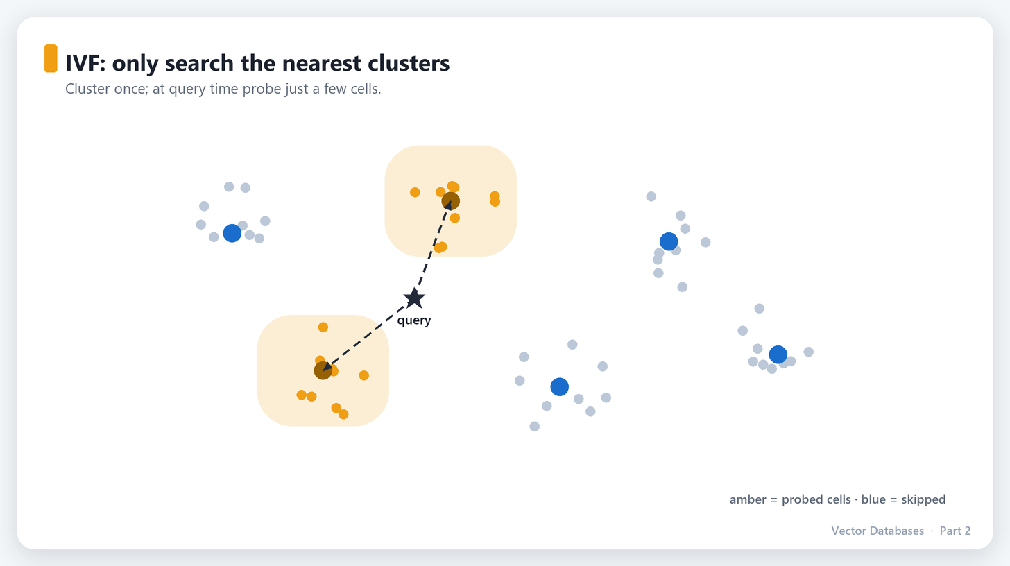
The knob: nprobe — how many clusters to actually open. nprobe=1 is fast but risky (the true neighbor might sit just across an aisle boundary). Higher nprobe = better recall, more work. Same recall↔speed dial, different shape.

The catch: those boundary misses are IVF’s weakness, and it needs a training step (running k-means on a representative sample) before you can insert.

Index C: Product Quantization — shrink the vectors (memory magic)

The previous two indexes reduce how many vectors you compare against. PQ attacks a different cost: the sheer size of the vectors.

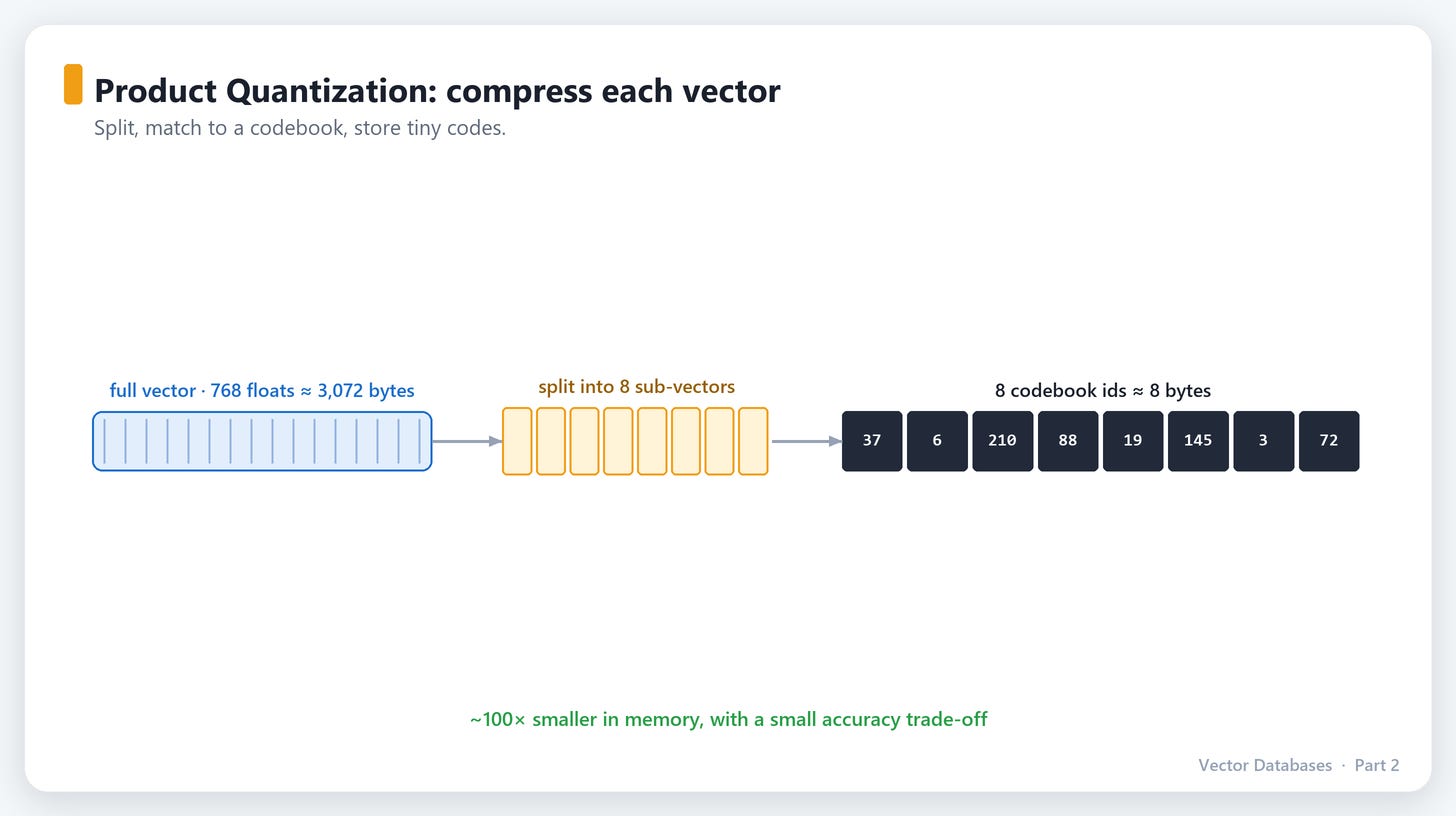
A 768-dim float32 vector is 768 × 4 = 3,072 bytes. A billion of them is ~3 terabytes of RAM. Ouch.

The intuition — compression by codebook. Chop each vector into chunks (say 8 sub-vectors of 96 dims). For each chunk position, learn a small “codebook” of ~256 representative sub-vectors. Now store each chunk as a single byte — the index of its closest codebook entry — instead of 96 floats.

Original chunk: [0.12, -0.44, ..., 0.09]  (96 floats = 384 bytes)
Codebook says:  "that's closest to entry #37"
Stored as:      37                          (1 byte)

That 3,072-byte vector can collapse to ~8–32 bytes — a 10–100× memory cut — and distances can be computed directly on the compressed codes. The cost is a little accuracy loss from the approximation.

The combo you’ll see in the wild: IVF + PQ — IVF narrows which vectors to look at, PQ makes each one tiny. It’s the classic recipe (FAISS’s IVFPQ, and the backbone of billion-scale, memory-constrained deployments). For disk-based scale, look up DiskANN, which keeps the graph on SSD instead of RAM.

Quick comparison

Layer 4: The rest of a real system

An index alone isn’t a database. Here’s what turns it into one.

Metadata filtering (harder than it looks)

Real queries are rarely pure similarity. They’re “most similar chunks, but only from documents in English, owned by this tenant, published after 2024.” So each vector carries a payload of metadata, and you filter on it.

The subtlety — when do you apply the filter?

Post-filtering: find nearest neighbors, then drop ones that fail the filter. Problem: if only 1% of data matches your filter, your top-100 might contain zero survivors. You asked for 10 and got nothing.
Pre-filtering: restrict to matching vectors first, then search. Correct, but a plain HNSW graph doesn’t naturally support “only walk through these nodes.”

Good databases (Qdrant is notably strong here) implement filterable ANN — the filter is fused into the graph traversal, so you get correct results without scanning everything. When you evaluate vector databases, how they handle filtered search is one of the most important real-world differentiators. Don’t skip it.

Sharding & replication (scaling out)

When data outgrows one machine:

Sharding splits vectors across nodes. A query fans out to all shards, each returns its local top-k, and the results are merged. This scales capacity and parallelizes search.
Replication copies each shard to multiple nodes for high availability and higher read throughput.

These give you horizontal scale and resilience — and they’re a big reason to choose a purpose-built vector DB over pgvector once you’re genuinely large. (Deployment details are Part 4.)

Persistence

The index may live in RAM for speed, but it must survive restarts. Systems persist via snapshots and/or a write-ahead log (WAL), rebuilding or memory-mapping the index on startup. “It’s all in memory” doesn’t mean “it’s lost on reboot.”

The tradeoff triangle (the mental model to keep)

Almost every decision in a vector database is a point inside one triangle:

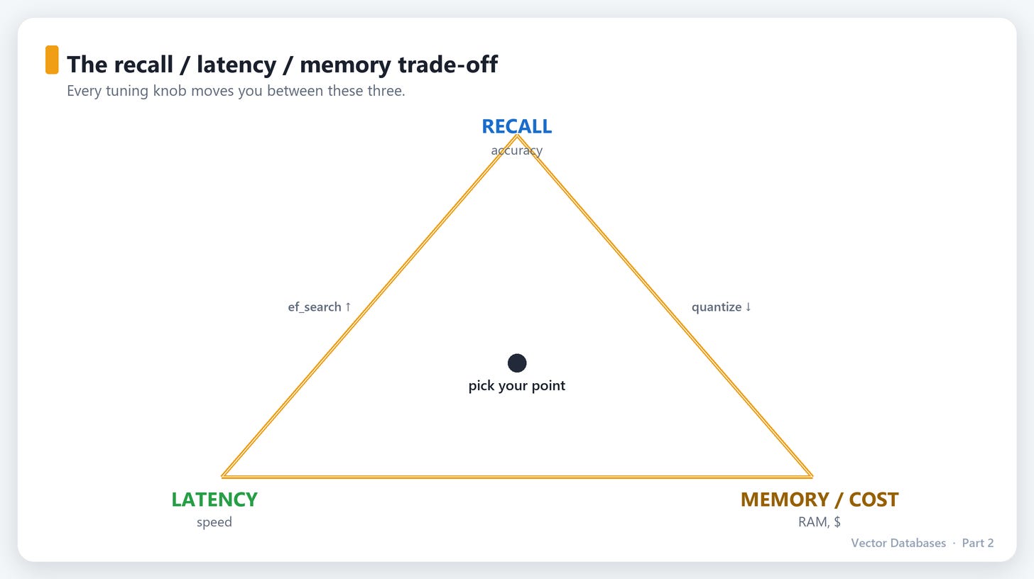
You cannot max all three. Every knob trades among them:

Raise ef_search / nprobe → ↑ recall, ↑ latency.
Add PQ compression → ↓ memory, ↓ recall slightly.
Raise M in HNSW → ↑ recall, ↑ memory.
Add replicas → ↑ throughput & availability, ↑ cost.

There is no universal “best config.” There’s only the best config for your recall target, latency budget, and wallet. Once you internalize this triangle, tuning stops being guesswork — you know which direction each dial moves you.

What’s next

You now understand the machine:

Distance metrics define “similar” — match the metric to your model (usually cosine).
Exact search dies at scale, so we accept Approximate Nearest Neighbor, measured by recall@k.
HNSW (navigate a graph), IVF (cluster and probe), and PQ (compress the vectors) are the three ideas behind nearly every index.
Real systems add metadata filtering, sharding, replication, and persistence — and everything is a point in the recall/latency/memory triangle.

Enough theory. In Part 3 we get our hands dirty: connecting to and querying real databases in Python — Chroma for a 60-second local start, pgvector for SQL lovers, Qdrant for production-grade filtering, and Pinecone for fully-managed — and we’ll assemble them into a complete RAG pipeline you can run yourself.

See you in Part 3 — bring a terminal.

Found the HNSW “express lanes” explanation useful? That one diagram is what finally made it click for a lot of people — feel free to share it.

Ramendra Singh Parmar

Discussion about this post

Ready for more?